Analysis Beginnings

MRC Clinical Sciences Centre

Bioinformatics Core Team

http://bioinformatics.csc.mrc.ac.uk/training.html

Getting hold of ChIP-seq data

• From public repositories
• From collaborators
• By sequencing some ChIP material!

Public Repositories

• Several public sources of ChIP-seq data exist.
• First concentrating on those acting as repositories.
  • GEO (Gene Expression Omnibus)
  • ENA (European Nucleotide Database)
  • SRA (Short Read Archive)

GEO (https://www.ncbi.nlm.nih.gov/geo/)

• GEO holds different types of biological datasets.
• Very popular for submission of data accompanying publication.
• Captures metadata,  processed files and raw data.
• GEO was not built for HTS data 

GEO - Quick Tour

SRA (www.ncbi.nlm.nih.gov/sra)

• NCBI's HTS specific repository.
• Sequencing specific metadata.
• Stores Raw data (in SRA format)
• SRA format - requires SRA Toolkit
• Lost then regained funding?

SRA - Quick Tour

ENA (https://www.ebi.ac.uk/ena)

• ENA acts as a european HTS repository.
• Mirrors much of SRA.
• Stores Raw data
• No SRA formats - fastq by default.

ENA - Quick Tour

Other Repositories

• Many repositories contain processed or unprocessed data.
• These typically are the result or a consortium's data release policies.
• Good example is Encode site. (https://www.encodeproject.org/)
• UCSC has many useful links to genomics data in various formats. (http://hgdownload.soe.ucsc.edu/downloads.html)

Time for a look at some code!

Data from Collaborators.

• Often collaborators will provide (very) processed data.
  • Saves time in transfer (raw data can be large).
  • Want to share some parts of data (but perhaps not all yet).
  • Analysis steps are in house only (so you could not replicate from raw data).

• Most basic format you will start with is fastq (but even that maybe processed.)

Data from Collaborators.

• Working with processed data types can be tricky. 
  • They may be unusual format.
  • They may have been processed in a way which confounds your analysis (repeat mapping strategies).
• Working from fastq will mean you understand how data has been processsed.
  • As long as you know how to process the data (collaborator's in-house methods may be unavailable).

Your own CSC data

• If you run high throughput sequencing at the Clinical Science Centre you will be delivered a path to your data in Fastq format. 

• The Bioinformatics Core will process optical data to base calls presented as Fastq.

• A member of the Core team will have assessed that your data meets minimal sequencing standards.

• Fastq maybe stored gzipped.

  • Many programs wont mind.

  • You will have to  unpack to view sequences manually.

Illumina Sequencing

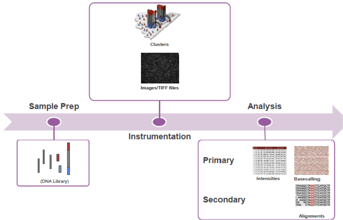
Overview

Basecalling quality Control

• This is undertaken by your local core team.
  • You wont be basecalling at CSC.
• This is only a brief overview of major quality steps.

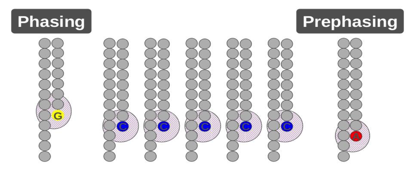
Phasing and pre-phasing.

•A small number of molecules in each cluster run ahead (prephasing) or fall behind(phasing) of the current cycle.

•Corrected for during base calling

Chastity Filtering

•Clusters filtered based on signal purity

•Only one cycle is allowed to have chastity value of < 0.6 for the first 25 cycles.

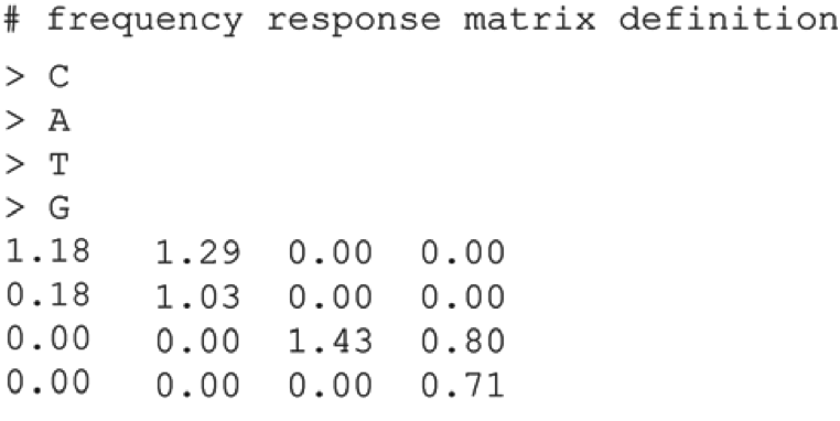
Intensity correction -

Lazer Cross Talk

•Two lasers are used to excite the dye attached to each nucleotide.

•The spectra from the four dyes overlap, such that the images are no independent.

•This cross-talk is resolved with a cross-talk matrix.

Quality control per base call

•Qscores = estimated probability of an incorrect base call

•Qscore = 10log10(e)

•Represented as ASCII characters to save space

• To get Phred score: (ASCII value – 33)

For more information on Phred scores come here

Bioinformatics Core Workflow

• Implemented in R (Mostly).
• Makes use of Illumina's software for basecalling.
• Allows for version control and some automation.
• Available on our MRC CSC Github.  (https://github.com/mrccsc/genomicsProcessing)

FastQ to Aligned Data

FastQ -> Aligned Data

• Fastq - Sequence of IP-ed fragments with base pair sequence confidence measures. 
• Often we want to know a bit more.
• Use knowledge of whole genome sequence to map our sequence reads to potential positions in genome.
• We need a few things then
  • Our FastQ files,
  • The whole genome sequence,
  • A tool to map fastQ sequences to genome sequence and report positions (and hopefully other useful information).

The Reference genome.

• Reference Genome available from many locations.
• Different assemblies
  • Major Revisisons - Change locations
  • Minor Revisions - Update annotation

Preparing the genome

• Concatenate chromsomes
• Attach ERCC spike FASTA
• Create an index for yout aligner

Choosing an aligner?

• Easy choise for ChIP-seq
  • Simple alignment
• Popular choices
  • BWA , BOWTIE2, subread
• Repeat mapping requires special alignment tools (CSEM).
  • And other special tools for peak calling (MOSAICS).

Rsubread for ChIP-seq

• subread combines speed with low memory usage.
  • STAR is fast but memory heavy.
• Part of a complement of interlinkning tools.
• Implemented in R (rsubread)

Mapping Quality Control

• Following alignment
  • Assess mapping rate.
  • Assess mapping quality/uniqueness.
• Technique specific expectations.
• Technique specific QC
  • Duplication rate for ChIP-seq.
• Should always review in IGV.

Viewing In IGV

ChIP-seq specific Alignment QC

• From the IGV Browser
  • Did we pile up of reads?
  • Where we expected?
  • Structured or random pileup? 
  • IGV has limit to window we see..
• Without a global view of the data we cant learn much more.
• Tools for assessment of ChIP-QC post alignment are available. i.e. Work on BAMs.

Post Alignment ChIP QC

Library Complexity and Duplication rate

• High duplication rate used to suggest low complexity starting material.
• With more read and high efficiency ChIP, not always true.
• Many duplicates found in peaks are shown to be false by paired end sequencing.

Reads in expected regions?

• Sets of known binding locations?
• Relationships to genes/enhancers?
• Enriched for repeats?
• We'll come back once we called peaks. (peaks)

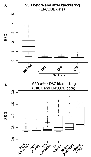
Reads in Blacklisted regions?

• As part of Encode project a list of regions with consistent ultra high signal was discovered.
• Anshul Kundaje created the DAC blacklist
• Blacklists can confound peak calling, QC metrics, HMM learning and comparison between samples

Signal Pile-up over genome

• It can be expected that
  • ChIP should have regions of high enrichment.
  • Input should have an even(ish) signal across genome.
• The standard deviation of the pile-up across genome gives a measure of genome wide peakiness.
• These metrics howver can be biased by Blacklisted regions.

Structured or Random?

• Did the example have random pile-up of reads
• A good TF peak shows structure.
  • "+" reads to 5' of peak
  • "-" reads to 3' of peaks
• Measuring this structure genome wide is a good measure of ChIP-quality

Measuring structure

• Identify start bp or reads on "+" and "-" strands.
• Shift "+" towards 3' by 1 bp
• Measure genome covered.
• Repeat shift and measure after every shift
• When 5' read end over 3' read ends around peaks we will get a lower than overage coverage.
• This shift size represents the fragment length.

Cross-coverage

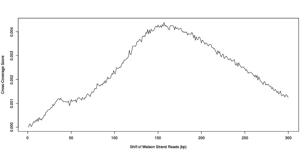
• Convert total coverage to cross-coverage scores to allow for comparison between samples (and regions)

Cross-Coverage Score  =(Coverage0 – CoverageN)/Coverage0

Frag_CC = Cross-coverage score at fragment length.

Time to look at some code!

Time for a Practical!